But, aren't neural networks 'magic'?

Nope. Just simple linear models.

Earlier we outlined the idea that all of classical statistics is just different ways to do linear modeling. While this is a little bit of an over-simplification, we can fix it using some statisical language: Nearly all of classical statistics can be approximated by linear models. If you'd like more information on this topic, please check out this web page on the subject, which covers quite a few of the most commonly-used statistical tests and includes examples with R code and links to additional information.

Just so we're all on the same page, recall that a "linear model" is just an equation of the form:

y = m * x + b

where y is the response variable, and x is the explanatory variable. In general, the simple linear model is a function that maps 'known' values of x (called the "independent variable") to corresponding 'unknown' values of y (called the "dependent variable", because the value of y 'depends on' the input value of x). For now, we can just think of x and y as real numbers (called "scalars"), but they don't have to be; they could be vectors, matrices, or tensors!

Remember that the simple linear model has two free parameters:

m - the slope of the line
In our case, the slope m is just a number that indicates the change in the response variable (y), given a change in the explanatory variable (x). Mathematically, the slope can be written as:
```
Δy/Δx
```
or you may have seen it written as:
```
(y1-y0)/(x1-x0)
```
for pairs (x0,y0), (x1,y1). Or, from calculus:
```
dy/dx
```
These all mean the same thing in this case. But as we aren't mathematicians, we don't need to worry too much about notation. For our simple case, m is just a number that we'll need to fit to our data, although in the more general case the slope can be a vector, matrix or tensor.
b - the y-intercept
The y-intercept b is the value of y when x=0. This is often called the "bias" in the machine-learning or AI world. Again, in our example, b is just a number that will be fit to a specific training data set. In higher-dimensional problems, b could be a vector, matrix or tensor, but we'll get to that later.

An important thing to remember is that the simple linear model does not describe a line! The linear model describes an infinite number of lines; one for each possible value of m and b! For example, the lines

y = 2.5 * x + -12.3

and

y = -5.8 * x + 58.0

are different lines, but they are the same linear model, just with different values for the free parameters, m and b.

But, how does this relate to "neurons"

The basic "neuron" in an artificial neural network can be thought of as a simple 'computational unit' that accepts inputs and produces an output. Mathematically, a 'neuron' is just a function, then. A neuron is typically drawn like the figure below.

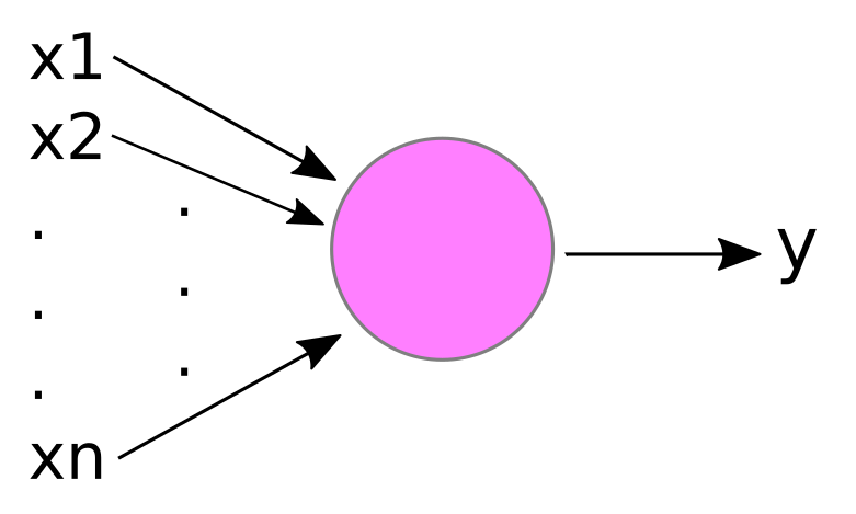
a neuron accepts inputs and produces an output

The inputs to this hypothetical pink neuron are labelled x1, x2,... xn, and the output is labelled y (hmm... sounds familiar?). In the figure, the vertical "..." just means that there can be 'any number' of inputs (ie, "n" can be any positive integer). Each input xi is 'attached' to the neuron by an incoming arrow (called an "edge" in network theory), and the output y is connected to the neuron by an outgoing arrow.

The purpose of the neuron is to apply some function to the collection of inputs, x1,x2,... xn, in order to produce the output y.

Theoretically, our neuron could apply any function to the inputs. While there are some 'fancy' neurons that apply fairly complex functions, in most cases y is a 'weighted sum' of the inputs x1,... xn. This is typically drawn like the image below.

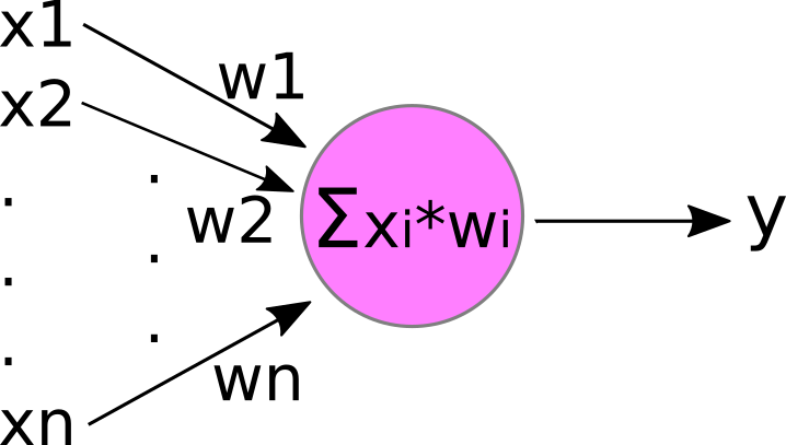
a neuron accepts inputs and sums them to produce an output

Here, we've labelled each incoming edge with a "weight" w1, w2,... wn. And 'inside' the neuron, we multiply each input xi by its incoming weight wi, and then sum the results to produce the output y.

As an example, let's consider the following neuron with two inputs:

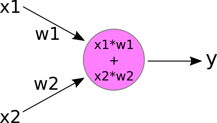
a neuron accepting 2 inputs and summing them to produce an output

If we plug in some values for the weights and inputs:

w1 = 2.5
w2 = -1.0
x1 = 1.0
x2 = 0.5

Then we can calculate the neuron's output y as:

y = 1.0 * 2.5 + 0.5 * -1.0 = 2.5 - 0.5 = 2.0

This little pink neuron is very close to the "perceptron", the first artificial neuron model that still forms the basis for nearly all of the neurons used today! There is still one small bit that we need to add, the "bias":

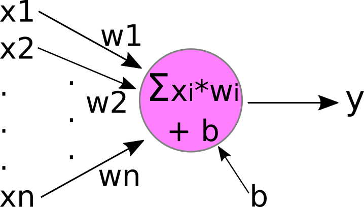
a neuron with multiple inputs and a bias term

Now our little neuron has a new free parameter, b, which it adds to the weighted-sum of the inputs x1,... xn. If you're still not convinced this is a linear model, let's simplify it a bit further to accept only a single input, x, and we'll change the name of the weight from "w" to "m":

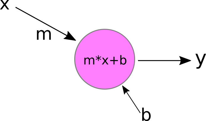
a neuron with a single input and a bias term

That looks exactly like a simple linear model to me! And adding more inputs doesn't make the model non-linear; it just makes x and m vectors instead of scalars!

Those of you who have heard about "activation functions" might be thinking that I've over-simplified our neuron by leaving out the activation function. Don't worry, we'll get to activation functions in a little bit, so if you don't know what they are, you will soon enough! While many of the earlier explanations of artificial neurons include the activation function as part of the neuron, most folks nowadays think of the activation function as an additional component or transformation that is applied to the neuron's output y afterwards. Incidentally (or perhaps not), this is how activation functions are actually implemented - as an additional component separate from and applied after the neuron's output.

But activation functions aside for now; I hope I've convinced you that the "neuron" in a "neural network" is really just a simple linear model, although it can be linear in more than 2 dimensions!

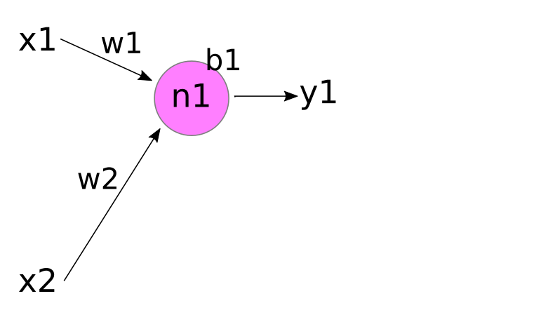
How are neurons connected into a "neural network"

Neurons connected to the same inputs form "layers", and the output of one layer can be connected to the input of another layer.

As we've seen above, a single neuron has extremely limited computational capacity; it is basically a simple linear model and nothing more. Even if we add an arbitrarily large number of inputs to the neuron, x1,... xn, the neuron is still just a linear model; it is just linear in a higher dimension! Maybe adding additional bias terms to our neuron could make it non-linear? Nope.

y = m * x + b1 + b2 + b3 + ... + bn

is still just a line, as you can see by substituting

c = b1 + b2 + b3 + ... + bn

And you thought you'd never use math in 'real life' :)

What makes the concept of the artificial neuron powerful is that you can connect many neurons together into a "network" to generate more interesting computations. How interesting? Recall from our previous discussion that a neural network should be able to approximate just about any computation you can do with real-valued numbers (and yes, that includes vectors, matrices and tensors of numbers).

The basic component of a neural network's "architecture" is the concept of a "layer". A "layer" in a neural network consists of all the neurons that are directly connected to the same inputs.

As an example, let's re-consider our basic single-neuron model with two inputs:

Recall that this 'neural network' is just a line in three dimensions; the neuron has two inputs, x1,x2, and produces output y1 by calculating:

y1 = w1*x1 + w2*x2 + b1

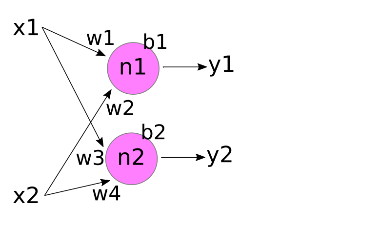
We can connect a new neuron, n2 to the same inputs, x1,x2, to create a network of two different linear models:

The two neurons, n1 and n2 have independent weights and bias terms, so the outputs y1,y2 are independent linear interpretations of the inputs, x1,x2. In this case, we have the computations:

y1 = w1*x1 + w2*x2 + b1
y2 = w3*x1 + w4*x2 + b2

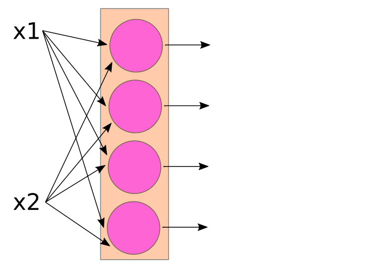
The neurons n1,n2 are connected to the same inputs, x1,x2, so they form a "layer". The "width" of this layer is 2, because there are 2 neurons in the layer. If we connect more neurons to the same inputs, we increase the width of the layer. For example:

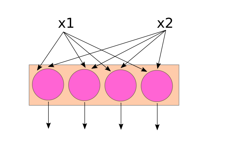
This neural network has a single layer (highlighted in light orange) with four neurons (pink circles) connected to the two inputs x1,x2. This little network produces four outputs (unlabelled), one for each of the neurons in the output layer. And no, it doesn't matter if you draw the network horizontally or vertically. The exact same network could be drawn like this:

a 4-neuron layer with two inputs, drawn vertically

Adding neurons to a layer increases the width of the layer. The "depth" of the network is increased by adding new layers, with the inputs of neurons in the new layer connected to the outputs of the preceding layer.

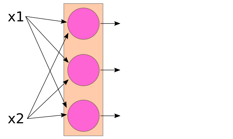
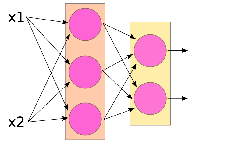
For example, let's take a simple 1-layer network with 2 inputs, x1,x2, and 3 neurons in the first layer (ie, the layer's width is 3).

Now let's add a new layer with 2 neurons (layer width = 2). In the 'perceptron' model, each of the neurons in the new layer is connected via inputs to every output of the previous layer. This is often referred to as a "densely connected" layer or a "dense" layer.

a 3-neuron layer with two inputs connected to a 2-neuron output layer

This new network now has two layers, so the network's "depth" is 2. The first layer's width is 3 (because it has 3 neurons), and the second layer's width is 2 (because it has 2 neurons). The network has 2 inputs, x1,x2, and two unlabelled outputs.

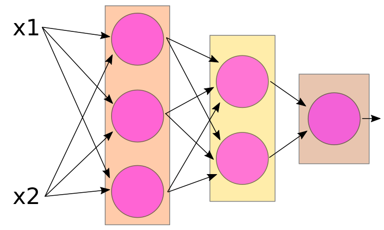
In nearly all cases, the number of outputs from a neural network is equal to the number of neurons in the final (output) layer of the network, so if we want a single output, we need to add a new layer to our network, consisting of a single output neuron:

a 3-layer neural network with 2 inputs and 1 output

In this particular network, the width of each layer decreases as we move from inputs toward output. This is fairly common but is certainly not universal; layer width can increase or decrease freely throughout the network.

Another thing you might notice about this network is that all the arrows point in the same direction - from inputs toward outputs. This type of network is called a "feed forward" network, from the idea that 'information' flows 'forward' through the network, starting from the inputs and moving through each layer in the network, until it reaches the output.

In all but a few very specialized cases, neural networks are "feed forward" networks. To make an inference, you supply the network with input data (in this case, values for x1 and x2), and the network proceeds to calculate 'layer-by-layer' from inputs to outputs, the 'inference' being the final output of the entire network.

During network 'training', the "forward pass" is used to make an inference from training data. The output from the forward pass is then compared to the 'true' output from the training data, using the loss function. The loss is then "back propagated" through the network in the reverse direction (from output toward inputs), using the chain rule to calculate gradients and update the network's parameter values (weights and biases). Hence, the training algorithm is called "back propagation".

So, connecting a bunch of linear units together makes a neural network non-linear?

Well... not quite.

While much of the power of neural networks comes from their "modular architecture" - the fact that you can connect many neurons together to increase their computational expressiveness - connecting a bunch of linear units together doesn't make them non-linear.

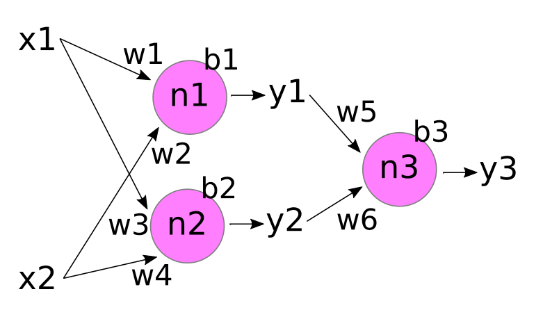
To illustrate this fact, let's consider the following simple neural network (I also promise that this is the most math we'll see in this course, and it's just algebra).

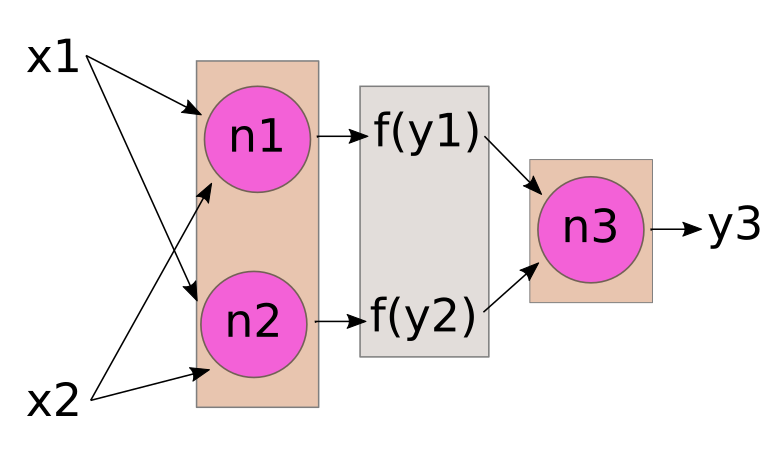
a simple neural network that's just linear

This little network has 2 inputs, x1,x2, and a single output y3. There are 3 total neurons in the network, 2 in the first layer (n1,n2) and one output neuron (n3). All the weights and bias parameters are shown, and we've labelled the intermediate outputs of neurons n1 and n2 as y1 and y2, respectively. Let's see how this network calculates it's output (y3).

The first layer in the network (n1,n2) accepts inputs x1,x2 and calculates intermediate outputs y1,y2 as follows:

y1 = w1*x1 + w2*x2 + b1
y2 = w3*x1 + w4*x2 + b2

Next, the second layer in the network (n3) accepts intermediate outputs y1,y2 and calculates y3:

y3 = w5*y1 + w6*y2 + b3

Now, we need to substitute for y1,y2 in the equation immediately above:

y3 = w5(w1*x1 + w2*x2 + b1) + w6(w3*x1 + w4*x2 + b2) + b3

Distribute...

y3 = w5w1*x1 + w5w2*x2 + w5b1 + w6w3*x1 + w6w4*x2 + w6b2 + b3

And combine terms...

y3 = (w5w1+w6w3)*x1 + (w5w2+w6w4)*x2 + w5b1 + w6b2 + b3

All those weights and bias terms are just constants, so we can let:

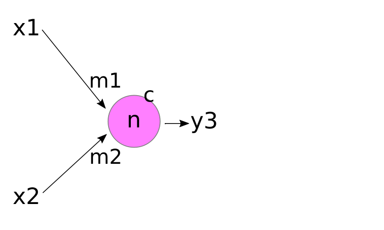
m1 = w5w1+w6w3
m2 = w5w2+w6w4
c  = w5b1 + w6b2 + b3

And substitute...

y3 = m1*x1 + m2*x2 + c

which is just a line in 3 dimensions, and is equivalent to the much simpler network shown below!

So, we just did a bunch of work to create a neural network with 9 parameters, 3 neurons and 2 layers, but it "collapses" into a simple, linear, 1-neuron model!

We need to add one more component to our neural network to make it capable of modeling non-linearity, and that is the "activation function". It is important to remember that, without non-linear activations, any neural network, no matter how complex, will always collapse to a simple linear model.

The "activation function" is any function that is applied to the outputs of a neural network layer. Sometimes the activation function is included in the definition of the neuron, but nowadays it is more common for people to define the activation function as a separate layer of the network, and as we'll see later on, this is typically how the activation function is actually implemented.

In nearly all cases, the activation function does not have any free parameters, so it doesn't increase the complexity of the network. What the activation function does do is apply a non-linear transformation to the outputs of the previous neural network layer, ensuring that the network doesn't collapse into a simple linear model.

The figure below shows our 3-neuron, 2-layer network with a non-linear activation function f(y) applied to the intermediate outputs from the first layer in the network.

a small neural network with nonlinear activation

Notice that the activation fuction is applied independently to each of the layer's outputs y1,y2, so it doesn't change the number of outputs from the layer.

You are pretty much free to choose any activation function you'd like, so long as it is differentiable (or back propagation won't work), and it is non-linear (or your model will collapse into a simple linear model).

Some of the more commonly-used activation functions are the sigmoid activation:

y = 1 / (1 + exp(-x))

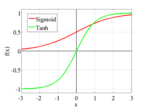
which produces an output between zero and one, and the hyperbolic-tangent (called "tanh") activation, which produces an output between -1 and +1. (The tanh function is a bit complicated, so we won't show it here.)

The following figure shows the output of sigmoid vs tanh activations on the Y-axis, for various input values on the X-axis.

sigmoid activation vs hyperbolic tangent

You can see that these functions are definitely not linear, so they will prevent our neural network from collapsing into a simple linear model.

But the activation function doesn't need to be S-shaped to work; even the very simple "rectified linear unit" or "ReLU" activation will make our neural network non-linear:

ReLU(x) = max(0,x)

ReLU activation is very simple. If x>0, ReLU(x)=x; otherwise, ReLU(x)=0 for all negative values of x. Those of you with a calculus background might notice that ReLU(x) is not technically differentiable; it has a singularity at x=0, but this is easily rectified (ha ha!) in practice by defining the derivative of ReLU(x) at x=0 to be zero (or 1, depending on the implementation).

The ReLU activation is extremely fast for a computer to calculate, and it performs well in practice, so it is one of the most commonly-used activation functions in neural networks today, particularly so for convolution networks, which are commonly used for image analysis.

Well, that's about it for neural networks: lots of neurons + non-linear activation functions = self-driving cars!

Okay, maybe not. But, given more than a few neurons and a simple non-linear activation function, you can construct a network capable of approximating nearly any mathematical function, given enough training data! And that's really all of the basic math underlying how AI works!